ANALYTICAL SCIENCES DECEMBER 2012, VOL. 282012 © The Japan Society for Analytical Chemistry
Rapid Communications
Relative Enrichment of Mo in the Radicle of Peanut Seed (Arachis hypogaea),Observed by Multi-elemental Imagining with LA-ICP-MS
Yanbei ZHU,*† Akiharu HIOKI,* Akihide ITOH,** Tomonari UMEMURA,*** Hiroki HARAGUCHI,***and Koichi CHIBA*
* National Metrology Institute of Japan (NMIJ), National Institute of Advanced Industrial Science and Technology (AIST), 1-1-1 Umezono, Tsukuba, Ibaraki 305–8563, Japan ** Faculty of Education, University of the Ryukyus, Azasenbaru, Nishihara, Okinawa 903–0213, Japan *** Department of Applied Chemistry, Graduate School of Engineering, Nagoya University, Furo-cho, Chikusa, Nagoya 464–8603, Japan
The distributions of eleven elements in a peanut seed were obtained by elemental imaging with laser ablation inductively coupled plasma mass spectrometry (LA-ICP-MS). The distribution of Mo was significantly different to those of other elements, such as K, P, and Mg. It was also confirmed that this typical enrichment of Mo was not dependent on the region where the peanut seed was planted. The enrichment of Mo was observed in the radicle of peanut seed, and was further confirmed by the isotopic ratio of Mo.
(Received October 4, 2012; Accepted November 12, 2012; Published December 10, 2012)
Over ten nutrient elements, such as Na, Mg, Ca, K, P, Fe, and Mo, are included in the dietary reference intakes set by Japan, USA, EU, UK, and Canada.1–5 This fact indicates that elemental analysis of the nutrient in food samples is a basic requirement for the quality management of food. On the other hand, the distribution of elements in biological samples is one of the major subjects of metallomics research as the integrated bio-metal science.6 Spatially resolved analysis with laser ablation (LA-) inductively coupled plasma mass spectrometry (ICP-MS) is an effective methodological approach for metallomics research in addition to bulk analysis.7 In recent years, LA-ICP-MS has been applied to elemental mapping in plant samples, such as bark,8 leaf,9–16 root,15–21 and grain.22,23 It is noteworthy that most of these applications have focused on the leaf and root for the uptake of nutritional elements or harmful heavy metals. Meanwhile, from the viewpoint that elemental mapping of seeds and grains will provide more information on mineral nutrition and food safety, such applications are still scarce.
Peanuts (Arachis hypogaea) are widely used as a food material all over the world. This could be attributed to the fact that peanuts are good source of mineral nutrients, such as Mg, P, K, Mn, Cu, and Mo, as well as organic nutrients, such as proteins, lipids, carbohydrates, vitamins, fatty acids, and dietary fibers.24 In the present experiment, the authors applied LA-ICP-MS to multi-elemental imaging of peanut seeds. A primary screening test on the target elements was carried out, covering all of the elements that have stable natural isotopes, from Li to Bi with the exception of rare gases. The signals of Th and U were also included in the screening test. The results showed that significant signal intensities could be obtained for C, Mg, P, K, Mn, Fe, Cu, Zn, Rb, Sr, Mo and Ba. Therefore, measurements of these elements were carried out for peanut seeds in the following experiments.
The LA-ICP-MS analysis was conducted by coupling a UP-213 (New Wave Research, USA) LA system and an Agilent 7700x (Agilent, Japan) ICP-MS instrument. In order to obtain a maximal sample, a spot size of 110 μm (the maximum of the present LA instrument) with the maximum output energy (ca. 3 mJ) was applied to the LA, where a typical depth of the ablation pits was approximately 50 μm. The LA sampling and the ICP-MS measurement were synchronized by sending the starting-signal from the LA system to the ICP-MS instrument. The elemental imaging was carried out using Graph-R software (developed by Mr. Tohru Itoh, Japan). The raw peanut seeds grown in Japan (Ibaraki) and China were respectively purchased from the market. The majority of peanut seeds analyzed were those produced in Japan, with those from China being analyzed to check the dependence of the elemental distribution on the region where peanuts were grown.
In order to check the natural elemental profiles, a peanut seed was manually broken and LA-ICP-MS measurements were carried out on one of the halves of the peanut seed containing the plumule (embryonic shoot), hypocotyl (embryonic stem), and the radicle (embryonic root). The elemental-images of 24Mg, 31P, 39K, and 95Mo in two samples are, representatively, shown in Fig. 1(a). It can be seen from Fig. 1(a) that the profiles of the elements depended on the shape of the sample, and relatively stronger signals of the elements were observed at some locations. Relatively stronger signal intensities of 31P and 39K were observed at the plumule and the radicle of both samples. Furthermore, it is noteworthy that relatively stronger signals of 95Mo were observed at the location of the radicle. This characteristic profile was found in the peanut seeds both from Japan and China and was not observed for other elements. In order to confirm the Mo profile, further measurements were carried out for the plumule, hypocotyl, and radicle parts.
† To whom correspondence should be addressed. E-mail: yb-zhu@aist.go.jp
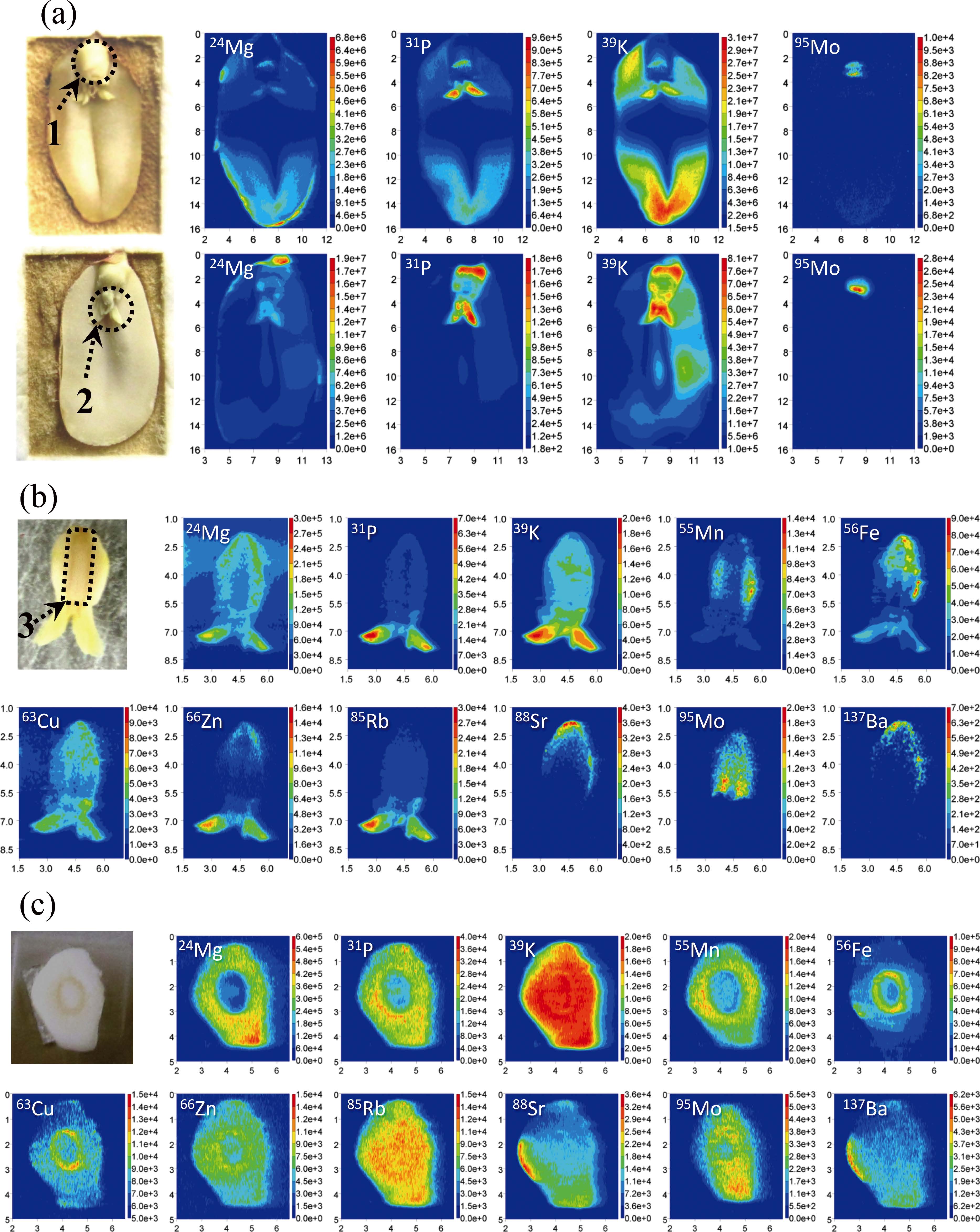
Fig. 1 Elemental images of peanut seed samples. The x-axis and y-axis give the relative distance (unit, mm).* Color scale, signal intensities (unit, CPS). (a) Results for whole peanut seed: the upper sample grown in Japan; the lower sample grown in China; 1, the radicle; 2, the plumule; 3, the hypocotyl. (b) The results for vertical-cut radicle, hypocotyl, and plumule.** (c) The results for horizontal-cut radicle and hypocotyl.*** *, Five replicates had been carried out parallel to each sample; the elemental image patterns are similar to one another. **, The cutting plane is parallel to the image in Fig. 1(a). ***, The cutting plane is perpendicular to the image, and is parallel to the bottom line in Fig. 1(a). Operating conditions: the energy fluency of the laser was approximately 31.6 J/cm2. Multi-elemental imaging of a sample was carried out by multiple line-scans with a line-to-line distance of 100 μm. The scanning speed for each line was 100 μm s–1. The ICP-MS instrument was working under the collision cell mode with 3.5 mL min–1 helium gas as the collision gas. The radio frequency power and the carrier gas of the ICP-MS were, respectively, 1500 W and 0.7 L min–1 argon gas. Measurements of the elements were carried out using the time-resolved mode, one point per peak, and the dwell time was 0.015 s, which permitted collection of 5 sets of data for each target element in one second.
The samples were separated manually, and cut with a stainlesssteel blade to obtain a flat surface for measurements. The correlation between the sample quantity and the signal intensity of 12C was investigated to confirm the usefulness of 12C as the internal standard. The correlation factor (R2) between the signal intensities of 12C and the square of the LA spot diameter (40, 65, 80, and 110 μm) was better than 0.99. Because the output energy of the laser was fixed, the sample quantity was in correlation to the LA spot diameter. These results showed that the signal intensity of 12C was in correlation to the sample quantity generated by the LA. Furthermore, the signal intensity of 12C was steady and independent of the parts (e.g., plumule, hypocotyl, and radicle) of the sample when the output energy and the spot diameter were fixed. Therefore, the signal intensities of 12C were used for normalization of the signal intensities of other elements in order to reduce the effect of any sampling quantity variation. The normalized signal intensity was calculated as 'Sele-i = Sele-i × SC-avg/SC-i, where 'Sele-i, Sele-i, SC-avg, and SC-i are the normalized signal intensity and the raw signal intensity of the element at data point i, the average signal intensity of 12C in the sample, and the raw signal intensity of 12C at data point i, respectively. The 12C-signals normalized elemental-images of 11 elements are shown in Figs. 1(b) and 1(c). It should be noted that the elemental-images in Figs. 1(b) and 1(c) were respectively obtained for vertical and horizontal cross sections of the plumule, hypocotyl, and the radicle parts of peanut seeds. It can be seen from Fig. 1(b) that the relatively stronger signal intensities of 24Mg, 31P, 39K, 66Zn, and 85Rb were observed at the plumule, while those of 55Mn and 56Fe were observed at the radicle and that of 65Cu were observed at both the plumule and the radicle. On the other hand, relatively stronger signal intensities for 88Sr and 137Ba were observed at the top of the radicle, while relatively stronger signal intensities for 95Mo were observed at the radicle parts around the hypocotyl.
The elemental-images in Fig. 1(c) were obtained for a horizontal-cut cross-section of the radicle and hypocotyl. It can be seen that relatively stronger signal intensities of 24Mg, 31P, 55Mn, and 66Zn were observed at the radicle, while those of 56Fe and 63Cu were observed at a narrow range around the hypocotyl. The signal intensities of 39K and 85Rb were generally equal at all parts of the hypocotyl and the radicle, while relatively stronger intensities of 88Sr and 137Ba were observed on one side of the radicle. Relatively stronger intensities of 95Mo were observed over a wide range, except for the outer side of the radicle and the center of the hypocotyl. This result further confirmed the results of 95Mo observed in Figs. 1(a) and 1(b). The signal intensities of 97Mo and 98Mo were also measured throughout the present work, and their results in all of the samples were similar to the parallel results of 95Mo.
The signal intensities of Mo isotopes and their ratios are, respectively, plotted in Figs. 2(a) and 2(b), where the data were obtained from one of the scanning lines in Fig. 1(b) at y-axis of 5.4 mm. It can be seen from Fig. 2(a) that the signal-intensity profiles of the Mo isotopes were similar to one another. Furthermore, it can be seen from Fig. 2(b) that the signal intensity ratios were relatively stable over the range from 35 to 55 s, and close to the isotopic ratios of natural Mo (97Mo/95Mo, 0.600, blue solid line; 98Mo/95Mo, 1.516, green solid line). These results proved that relatively stronger signal intensities for Mo isotopes did not suffer from significant spectral interferences.
A quantification analysis with ICP-MS after microwave assisted acid digestion using HNO3, H2O2, and HF was carried out on the peanut seeds ground in Japan, which were separated into two parts, i.e. the cotyledon and all other parts containing
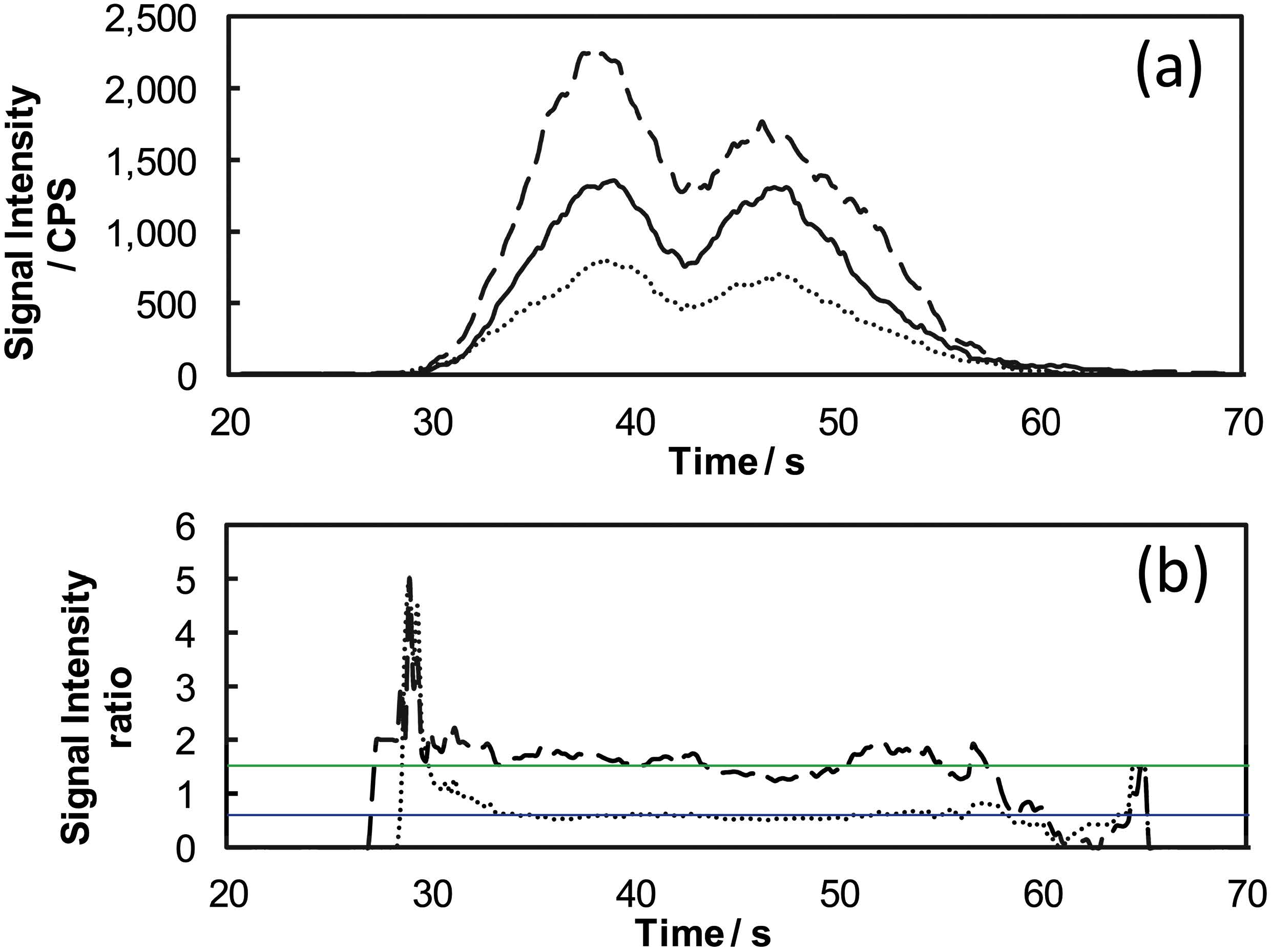
Fig. 2 Signal intensities and ratios of Mo isotopes observed from a scanning line of vertical-cut radicle and hypocotyl. (a) Signal intensity: solid line, 95Mo; dotted line, 97Mo; dashed line, 98Mo. (b) Signal intensity ratio: dotted line, 97Mo/95Mo; dashed line, 98Mo/95Mo; blue solid line, natural isotope ratio of 97Mo/95Mo; green solid line, natural isotope ratio of 98Mo/95Mo.
the radical, the plumule, and the hypocotyl. The concentrations of 18 elements including all of the elements shown in Fig. 2 were determined. The concentrations of most elements were generally equivalent in the two parts of each seed. However, the concentration of Mo in the part containing the radical was significantly higher than that in the cotyledon, by ca. 5-fold. The concentrations of Mo in the part containing the radical and that in the cotyledon were 2.2 (1.1) mg kg-1 and 0.56 (0.25) mg kg-1, respectively, while the values in the brackets are the standard deviations obtained from the results of 7 peanut seeds. These results confirmed the relative enrichment of Mo in the radical of peanut seeds, as observed in the present work. The quantification results of the elements in peanut seeds will be reported in detail in an article following the present work.
Conclusions
The enrichment of Mo in the radicle of peanut seed was observed and confirmed from the results in the present experiment. However, according to the authors’ knowledge, the mechanism for this kind of Mo enrichment is not clear to date. Therefore, further research on the speciation of Mo in peanut seeds is required and could provide important information help to understand this phenomenon. Some reports have shown that the deficiency of Mo in the soil limited the yield of plants,25 and the distribution of Mo was relatively enriched in the roots of whole plants.26 It is found in the present work that Mo was enriched in the radicle (i.e. the embryonic root) of the peanut seed; this might be relative to the function of nitrate reductase which requires Mo for its activity.27
It is known that peanut seeds are one of the nutritional sources that is abundant in Mo,24 the present results showed that the Mo content in peanut seed is enriched in the radicle. This characteristic distribution of Mo might be applied to develop a Mo-supplement food using the peanut radicle.
In the present work, discussion on the elemental imaging was carried out based on the signal intensities of the element, which indicated the relative distribution of the elements in the sample. Some reports showed that LA-ICP-MS with matrix-matching calibration could provide quantitative imaging results of the elements in plant samples.11,17 The authors are trying to establish a quantitative imagining method for the elements in peanuts by LA-ICP-MS.
Acknowledgements
The present research was partially supported by Grant-in-Aid for Scientific Research (B) (No. 21350041) from the Japan Society for the Promotion of Science. The present authors express sincere gratitude to Mr. Alex Groombridge (The University of Sheffield) for his kind advice to improve the English expressions in the manuscript. The present authors also express sincere gratitude to Mr. Tohru Itoh for providing free software, Graph-R.
References
- “Dietary Reference Intakes for Japanese-2010”, Ministry of Health, Labour and Welfare of Japan, http://www.mhlw. go.jp/shingi/2009/05/s0529-4.html, accessed 14 April 2012.
- “Dietary Reference Intakes: Recommended Intakes for Individuals”, National Academy of Sciences, Institute of Medicine, Food and Nutrition Board, USA, http://www. iom.edu/Activities/Nutrition/SummaryDRIs/~/media/Files/ Activity%20Files/Nutrition/DRIs/New%20Material/ 5DRI%20Values%20SummaryTables%2014.pdf, accessed 14 April 2012.
- “Safe Upper Intake Levels for Vitamins and Minerals”, Scientific Committee on Food, EU, http://ec.europa.eu/food/ food/labellingnutrition/supplements/documents/denmark_ annex2.pdf, accessed 14 April 2012.
- “Safe Upper Levels for Vitamins and Minerals”, Expert Group on Vitamins and Minerals, UK, http://www.food. gov.uk/multimedia/pdfs/vitmin2003.pdf, accessed 14 April 2012.
- “Dietary Reference Intakes, Reference Values for Elements”, Health Canada, http://www.hc-sc.gc.ca/fn-an/nutrition/ reference/table/ref_elements_tbl-eng.php, accessed 14 April 2012.
- H. Haraguchi, J. Anal. At. Spectrom., 2004, 19, 5.
- R. Lobinski, J. S. Becker, H. Haraguchi, and B. Sarkar, Pure Appl. Chem., 2010, 82, 493.
- M. Siebold, P. Leidich, M. Bertini, G. Deflorio, J. Feldmann, E. M. Krupp, E. Halmschlager, and S. Woodward, Anal.Bioanal. Chem., 2012, 402, 3323.
- T. Punshon, B. P. Jackson, P. M. Bertsch, and J. Burger, J. Environ. Monit., 2004, 6, 153.
- M. Galiová, J. Kaiser, K. Novotný, M. Hartl, R. Kizek, and P. Babula, J. Microsc. Res. Tech., 2011, 74, 845.
- B. Wu, Y.-X. Chen, and J. S. Becker, Anal. Chim. Acta, 2009, 633, 165.
- M. Galiová, J. Kaiser, K. Novotný, J. Novotný, T. Vaculovicˇ, M. Liška, R. Malina, K. Stejskal, V. Adam, and R. Kizek, Appl. Phys. A, 2008, 93, 917.
- J. Kaiser, M. Galiová, K. Novotný, R. Cˇ ervenka, L. Reale, J. Reale, J. Reale, J. Nototný, M. Liška, O. Samek, V. Kanický, A. Hrdlicˇka, K. Steiskal, V. Adam, and R. Kizek, Spectrochim. Acta, Part B, 2009, 64, 67.
- B. Wu, M. Zoriy, Y.-X. Chen, and J. S. Becker, Talanta, 2009, 78, 132.
- J. S. Becker, R. C. Dietrich, A. Matusch, D. Pozebon, and V. L. Dressler, Spectrochim. Acta, Part B, 2008, 63, 1248.
- A. Hanc, D. Barałkiewicz, A. Piechalak, B. Tomaszewska, B. Wagner, and E. Bulska, Int. J. Environ. Anal. Chem., 2009, 89, 651.
- A. B. Moradi, S. Swoboda, B. Robinson, T. Prohaska, A. Kaestner, S. E. Oswald, W. W. Wenzel, and R. Schulin, Environ. Experi. Botany, 2010, 69, 24.
- J. Santner, H. Zhang, D. Leitner, A. Schnepf, T. Prohaska, M. Puschenreiter, and W. W. Wenzel, Environ. Experi. Botany, 2012, 77, 219.
- B. Wu, I. Susnea, Y.-X. Chen, M. Przybylski, and J. S. Becker, Int. J. Environ. Anal. Chem., 2011, 307, 85.
- B. Klug, A. Specht, and W. J. Horst, J. Exp. Bot., 2011, 62, 5453.
- J.-Y. Shi, M. A. Gras, and W. K. Silk, Planta, 2009, 229, 945.
- Y.-X. Wang, A. Specht, and W. J. Horst, New Phytol., 2011, 189, 428.
- I. Cakmak, M. Kalayci, Y. Kaya, A. A. Torun, N. Aydin, Y. Wang, Z. Arisoy, H. Erdem, A. Yazici, O. Gokmen, L. Ozturk, and W. J. Horst, J. Agric. Food Chem., 2010, 58, 9092.
- Y. Kagawa, “Tables of Food Composition”, 2011, Kagawa Education Institute of Nutrition Pub., Sakado, Saitama, 44.
- M. Yu, C.-X. Hu, and Y.-H. Wang, Plant Soil, 2002, 245, 287.
- S. Jongruaysup, B. Dell, R. W. Bell, G. W. O’Hara, and J. S. Bradley, Ann. Bot., 1997, 79, 67.
- M. Anke and M. Seifert, Acta Biol. Hung., 2007, 58, 311.
JOURNAL OF CHEMICALEDUCARION
Technology Report pubs.acs.org / jchemeduc
Three-Dimensional Visualization of Wave Functions for Rotating Molecule: Plot of Spherical Harmonics
Shin-ichi Nagaoka,*,† Hiroyuki Teramae,‡ and Umpei Nagashima#
†Department of Chemistry, Faculty of Science and Graduate School of Science and Engineering, Ehime University, Matsuyamabr 790-8577, Japan
‡Faculty of Science, Josai University, 1-1 Keyakidai, Sakado 350-0295, Japan
#National Institute of Advanced Industrial Science and Technology, 1-1-1 Umezono, Tsukuba 305-8568, Japan
Supporting Information
ABSTRACT
Wave functions for rotating diatomic molecules (spherical harmonics) were three-dimensionally visualized by using Graph-R in tandem with Excel.
KEYWORDS
Second-Year Undergraduate, Physical Chemistry, Computer-Based Learning, Quantum Chemistry
At an early stage of learning quantum chemistry, undergraduate students usually encounter the concepts of the particle in a box, the harmonic oscillator, and then the particle on a sphere. Rotational levels of a diatomic molecule can be well approximated by the energy levels of the particle on a sphere. Wave functions for the particle in a one-dimensional box and the one-dimensional harmonic oscillator are functions of one coordinate and are easily drawn using Microsoft Excel1 due to rapid advancements in computer hardware and software. In contrast, wave functions for the particle on a sphere, that is, for a rotating diatomic molecule, are functions of two angular coordinates (spherical harmonics) and drawing them is much more difficult than drawing wave functions of one coordinate. In drawing them, it is necessary to plot contours on the surface of a sphere, but it is not possible to do this with Excel alone. Accordingly, the wave function for the particle on a sphere is typically drawn as a plot at a certain set value for one angular coordinate1,2 or as a plot on the rectangular coordinates of the two angles.3 It would be more beneficial to students if they could create, by themselves, three-dimensional polar plots of the wave functions for the particle on a sphere so that they could visualize the overall shapes of the wave functions for a rotating diatomic molecule.
In this report, we present a method for drawing the contour plots of the particle’s wave functions on the surface of the sphere by using Graph-R4 in tandem with Excel. Most students are familiar with Excel, so it is widely used in practical training on quantum chemistry.1,5,6 Graph-R is free software with which the contours can be plotted on the surface of the sphere. One can quickly download the software and run it easily from a PC desktop. Although free Graph-R does not support all of the functions provided in commercially available mathematical or plotting packages (such as Mathematica and Mathcad), it does support a number of functions commonly used by students.
The wave functions for the particle on a sphere are spherical harmonics and have a general form Yl,m(θ,ϕ), where l = 0, 1, 2, ... and m = −l, −l + 1, ..., l − 1, l and m are quantum numbers, and θ and ϕ are the colatitude and azimuth, respectively, in a spherical polar coordinate system.1 A general representation of Y1,0,7 with a dumbbell shape familiar to students, is shown in Figure 1. It would pass smoothly into the plot of the 2p atomic
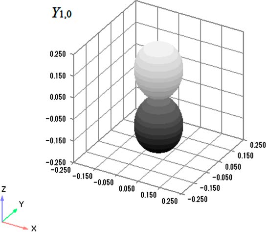
Figure 1. Y1,0 with dumbbell shape. In this representation, the distance between the origin and a point on the surface equals the value of |Y1,0|2 at that point. Plot was drawn using Graph-R in tandem with Excel; color on surface was gradated from black to white to clearly illustrate surface shape.
orbital.8 Its rotatable three-dimensional image, together with those of other Yl,m, is available elsewhere by using a free browser plug-in.9 However, a different type of representation for spherical harmonics is needed for the wave functions of the particle on a sphere because the radius of the sphere is fixed. The radius corresponds to the bond length of the rotating diatomic molecule.
The method for drawing the contour plot is explained in detail in the Supporting Information, and several sample plots are provided. Briefly, as input, Graph-R requires a set of x, y, and z Cartesian coordinates and the corresponding functional value given in a csv file. Accordingly, a set of θ and ϕ angular coordinates is converted into a set of x, y, and z Cartesian coordinates, and the corresponding value of Yl,m is calculated with Excel and saved in a csv file. Graph-R is then initiated, the csv file is opened, and the contour lines on the surface of the sphere are displayed on the monitor screen.
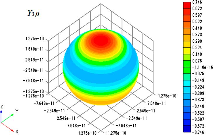
As an example, the plot of Y1,0 is shown in Figure 2. The radius of the sphere equals the bond length of an HCl molecule
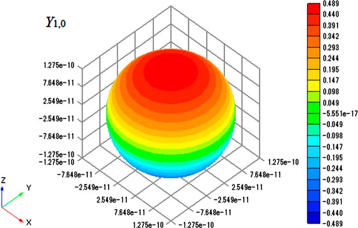
Figure 2. Contour plot of Y1,0 on surface of sphere with radius of
1.2746 × 10⁻¹⁰ m.
(1.2746 × 10⁻¹⁰ m),10 so the plot shows an excited-state wave function for a rotating HCl molecule. The node of the spherical harmonics is clearly seen in the figure. With Graph-R, one can change the perspective so that the plot can be viewed from a different angle and can rotate the plot freely (three-dimensional visualization). Thus, a drawing of Yl,m as a contour plot on the surface of the sphere should greatly promote the understanding of the concept of the particle on a sphere and of the wave functions for the corresponding diatomic molecular rotation. Therefore, using of Excel along with Graph-R is a good way to improve practical drawing training.
ASSOCIATED CONTENT
Supporting Information
Method for drawing contour plots, Yl,m contour plots on surface of sphere with radius of 1.2746 × 10⁻¹⁰ m, and Excel and csv files. This material is available via the Internet at http://pubs. acs.org.
AUTHOR INFORMATION
Corresponding Author
*E-mail: nagaoka@ehime-u.ac.jp.
Notes
The authors declare no competing financial interest.
ACKNOWLEDGMENTS
We express our sincere gratitude to Mr. Tohru Itoh of the Graph-R Project for permitting us to use Graph-R for this work.
REFERENCES
- Walters, V.; de Paula, J.; Atkins, P. Explorations in Physical Chemistry, 2nd ed.; Oxford University Press: Oxford, 2007.
- Miles, D. G., Jr.; Francis, T. A. J. Chem. Educ. 2001, 78, 405−408.
- McDermott, T.; Henderson, G. J. Chem. Educ. 1990, 67, 915−917.
- http://software-dev.jpn.org/download/GraphR/GraphR159e. zip, http://software-dev.jpn.org/download/GraphR/GraphR_ Manual_en.zip, and http://www.graph-project.com (accessed Apr 2013).
- Quin, C. M. Computational Quantum Chemistry: An Interactive Guide to Basis Set Theory; Academic Press: London, 2002.
- Nagaoka, S.; Teramae, H.; Nagashima, U. Chem. Lett. 2012, 41, 9−14 (Highlight Review).
- Lang, P. L.; Towns, M. H. J. Chem. Educ. 1998, 75, 506−509.
- Ellison, M. J. Chem. Educ. 2004, 81, 158 and http://www. chemeddl.org/alfresco/service/org/chemeddl/symmath/app?app_id= 48&guest=true (accessed Apr 2013).
- Wolfram Demonstrations Project. http://demonstrations. wolfram.com/SphericalHarmonics (accessed Apr 2013).
- Herzberg, G. Molecular Spectra and Molecular Structure I. Spectra of Diatomic Molecules; Van Nostrand Reinhold: New York, 1950; p 534.
©2013 American Chemical Society and Division of Chemical Education, Inc.